Sistemi Fisici

Introduzione

$$\Large \xrightarrow[\text{ causa (INPUT) }]{\text{ sollecitazione }} \boxed{\text{SISTEMA}} \xrightarrow[\text{ effetto (OUTPUT) }]{\text{ risposta }}$$

Il sistema applica una trasformazione di segnali.

Sistemi monodimensionali tempo-continui

$$\Large \xrightarrow[\text{ (INPUT) }]{x(t)} \boxed{\mathcal{T}} \xrightarrow[\text{ (OUTPUT) }]{y(t)}$$

Un sistema monodimensionale tempo-continuo opera una trasformazione su segnali di tipo tempo-continui. Lo schema di sopra si formalizza con la scrittura:

$$y(t) = \mathcal{T} [x(\alpha); \,t] = \mathcal{T}[x(t)] \quad\forall t \in \R$$

Esempio: corrente di un circuito elettrico:

$$i(t) = \mathcal{T}[v(t)] = \frac{v(t)}{R}$$

Proprietà dei sistemi tempo-continui

Lineare: vale il principio di sovrapposizione degli effetti.

$$x(t)=\alpha x_1(t) + \beta x_2(t) \implies y(t)=\alpha \mathcal{T} [x_1(t)] +\beta \mathcal{T} [x_2(t)]$$

Stazionario: il sistema è tempo invariato.

$$y(t) = \mathcal{T} [x(t)] \implies \mathcal{T}[x(t-t_0)] = y(t-t_0)$$

Causale: rispetta il nesso causa-effetto. L’output si ottiene considerando l’input solamente negli istanti di tempo passati.

$$y(t) = \mathcal{T} [x(\alpha), \, \alpha \leq t ; \,t]$$

Istantaneo o senza memoria: l’output ad un dato istante si ottiene considerando l’input solamente nel medesimo istante.

$$y(t) = \mathcal{T} [x(\alpha), \, \alpha = t]$$

Un sistema istantaneo può essere anche denominato come statico (non dinamico), puramente algebrico o combinatorio (nel caso di un sistema digitale).

Stabile: la limitatezza del dominio dell’input implica un dominio limitato anche per l’output.

$$|x(t)| \leq M \implies |y(t)|\leq N,\; \forall t$$

La stabilità di un sistema indica la capacità dello stesso di reagire con variazioni limitate a perturbazioni nello stato iniziale (o dell’ingresso).

Invertibile: scambiando l’input con l’output continua ad esistere una trasformazione che leghi tali funzioni.

$$\exist \mathcal{T}^{-1} \; \text{ t.c. } \; x(t)=\mathcal{T}^{-1}[y(t)]$$

Sistemi monodimensionali tempo-discreti

$$\Large \xrightarrow[\text{ (INPUT) }]{x[n]} \boxed{\mathcal{T}} \xrightarrow[\text{ (OUTPUT) }]{y[n]}$$

Un sistema monodimensionale tempo-discreto opera una trasformazione su segnali di tipo tempo-discreti. Lo schema di sopra si formalizza con la scrittura:

$$y[n] = \mathcal{T}\big[x[\alpha]; \,n\big] = \mathcal{T}\big[x[n]\big] \quad\forall n \in \Z$$

Proprietà sistemi tempo-discreti

Le proprietà sono pressoché identiche a quelle dei segnali tempo-continui.

Lineare: vale il principio di sovrapposizione degli effetti.

$$x(t)=\alpha x_1[n] + \beta x_2[n] \implies y[n]=\alpha \mathcal{T} [x_1[n]] +\beta \mathcal{T} [x_2[n]]$$

Stazionario: il sistema è tempo invariato.

$$y[n] = \mathcal{T} [x[n]] \implies \mathcal{T}[x[n-n_0]] = y[n-n_0]$$

Causale: rispetta il nesso causa-effetto. L’output si ottiene considerando l’input solamente negli istanti di tempo passati.

$$y[n] = \mathcal{T} [x[\alpha], \, \alpha \leq t ; \,t]$$

Istantaneo o senza memoria: l’output ad un dato istante si ottiene considerando l’input solamente nel medesimo istante.

$$y[n] = \mathcal{T} [x[\alpha], \, \alpha = t]$$

Stabile: la limitatezza del dominio dell’input implica un dominio limitato anche per l’output.

$$|x[n]| \leq M \implies |y[n]|\leq N,\; \forall t$$

Invertibile: scambiando l’input con l’output continua ad esistere una trasformazione che leghi tali funzioni.

$$\exist \mathcal{T}^{-1} \; \text{ t.c. } \; x[n]=\mathcal{T}^{-1}[y[n]]$$

Sistemi LTI

Un sistema LTI (lineare tempo-invariato) o SLS (sistema lineare stazionario) gode delle seguenti proprietà sopra citate:

• Linearità: principio di sovrapposizione degli effetti
• Stazionarietà: tempo-invarianza

L’istante iniziale di un sistema tempo-invariato si può sempre assumere nullo: $t_0=0$.

Un sistema LTI monodimensionale tempo-continuo è descritto da risposta impulsiva $h(t)$ e risposta in frequenza $H(f)$. Ulteriore discriminante è il numero di ingressi/uscite:

• multi-variabile o MIMO: Multi-Input Multi-Output
• singola variabile o SISO: Single-Input Single-Output

I paragrafi che seguono trattano dunque sistemi LTI SISO.

---

I sistemi LTI possono essere sia tempo-continui che tempo discreti.

Risposta Impulsiva

$$\Large \xrightarrow{\delta(t)} \boxed{\mathcal{T}} \xrightarrow{h(t)}$$

La risposta impulsiva per sistemi tempo-continui è la risposta all’impulso Delta di Dirac: $h(t) = \mathcal{T}[\delta(t)]$. Dunque $h(t)$ consente di calcolare l’output a partire da un qualsiasi input.

$$y(t)=\mathcal{T}[x(t)]=\int_{-\infty}^{\infty} x(\tau) \mathcal{T} [\delta(t-\tau)]d\tau = \int_{-\infty}^{\infty} x(t)h(t-\tau)d\tau = x(t) \otimes h(t)$$

Il sistema è lineare, l’integrale rappresenta una somma.

Il sistema è causale $\iff h(t) = 0$ per $t<0$. Il sistema è stabile $\iff \int_{-\infty}^{\infty} |h(t)| \leq M$

---

Nel campo dei sistemi tempo-discreti, la funzione Delta di Dirac non esiste: viene approssimata dall’impulso unitario $\delta [n]$.

$$\Large \xrightarrow{\delta[n]} \boxed{\mathcal{T}} \xrightarrow{y[n]}$$

La risposta impulsiva è utile per determinare l’output quando è noto l’input. Si applica l’operatore di convoluzione.

$$\large y[n] = \mathcal{T} \bigg[\delta [n]\bigg] \implies x[n]=x[n]\ast\delta [n]$$

Si può dimostrare che:

$$y[n]=\mathcal{T}_{\rm LTI} \biggl[ x[n]\biggr]=\sum_{m=-\infty}^\infty x[k]h[n-k]$$

Il sistema è causale $\iff h[n]=0$ per $n<0$. Il sistema è stabile $\iff \sum_{n=-\infty}^{+\infty} |h[n]|=M <\infty$

Risposta in Frequenza

$$\Large H(f) = \mathcal{F}[h(t)]$$

La risposta in frequenza è la trasformata di Fourier della risposta impulsiva.

$$y(t)=x(t) \ast h(t) \implies Y(f)=X(f)\cdot H(f) \implies H(f)=\frac{Y(f)}{X(f)}$$

Il dominio di esistenza della risposta in frequenza è l’insieme dei numeri complessi $\C$. Si definiscono il modulo e l’argomento della risposta in frequenza come:

1. risposta in ampiezza: $A(f) = |H(f)|$
2. risposta in fase: $\Theta(f) = \arg(H(f))$

$$H(f)=A(f)e^{j\Theta(f)} \in \C$$

---

La risposta in frequenza è la trasformata di Fourier della risposta impulsiva anche per i sistemi tempo-discreti. La risposta in frequenza dei sistemi tempo-discreto hanno periodo $1/T$.

$$\large \overline{H}(f) =\mathcal{F}[h[n]]=\sum_{n=-\infty}^\infty h[n]e^{-j2\pi fnT}=\frac{\overline{Y}(f)}{\overline{X}(f)}$$

Sistemi in cascata

Questo paragrafo analizza segnali tempo-continui, ma i ragionamenti fatti potrebbero essere riportati per segnali tempo-discreti.

$$\Large \xrightarrow{x(t)} \boxed{\mathcal{T}_1} \xrightarrow{y(t)} \boxed{\mathcal{T}_2} \xrightarrow{z(t)}$$

Dunque la funzione in output è:

$$z(t)=y(t)\ast h_2(t)=\bigg[ x(t)\ast h_1(t) \bigg]\ast h_2(t)$$

Concettualmente equivalente ai due schemi a blocchi che seguono:

$$\xrightarrow{x(t)} \boxed{h_1(t)\ast h_2(t)} \xrightarrow{z(t)} \quad ; \quad \xrightarrow{X(f)} \boxed{H_1(f)H_2(f)} \xrightarrow{Z(f)}$$

La cascata è invertibile. Con $\widetilde{y}(t) \neq y(t)$ perché l’operatore di convoluzione non gode della proprietà commutativa.

$$\Large \xrightarrow{x(t)} \boxed{\mathcal{T}_2} \xrightarrow{\widetilde{y}(t)} \boxed{\mathcal{T}_1} \xrightarrow{z(t)}$$

Esempio di sistema a cascata

Si consideri un sistema lineare e stazionario. Sia $x(t)$ il segnale in ingresso ed $y(t)$​ quello in uscita.

Il sistema è composto da un nodo sommatore:

$$z(t) = x(t)+y(t)$$

In seguito, sono disposti due dispositivi in cascata che eseguono le trasformazioni:

$$\begin{aligned} w(t) &= \frac{1}{2\pi A} \frac{dz(t)}{dt}\\ \\ y(t) &= \frac{1}{2\pi A} \frac{dw(t)}{dt} \end{aligned}$$

con $A=2 \cdot 10^4$ Hertz, ovvero 20 kHz e il segnale $y(t)$ che poi “torna indietro” al sommatore iniziale.

---

Si può formalizzare quanto scritto sopra con un paio di sistemi di equazioni:

$$\begin{cases} z(t) = x(t) + y(t)\\ w(t) = \frac{1}{2\pi A} \frac{dz(t)}{dt}\\ y(t) = \frac{1}{2\pi A} \frac{d w(t)}{dt}\\ \end{cases} \Large \xrightarrow{\mathcal{F}} \normalsize \begin{cases} Z(f) = X(f) + Y(f)\\ W(f) = \frac{1}{2\pi A} Z(f) j2\pi f = \frac{jf}{A} Z(f)\\ Y(f) = \frac{1}{2\pi A} W(f) j2\pi f = \frac{jf}{A} W(f)\\ \end{cases}$$

Si può ottenere così la definizione di $Y(f) = \mathcal{F}[y(t)]$ “in funzione” della trasformata dell’ingresso del sistema:

$$\begin{aligned} Y(f) &= \frac{jf}{A} W(f) = \frac{jf}{A} \bigg(\frac{jf}{A} Z(f)\bigg) =\\ &= \frac{j^2 \cdot f^2}{A^2} \bigg(X(f) + Y(f)\bigg)\\ \implies & Y(f)\bigg[ 1+ \frac{f^2}{A^2}\bigg] = -\frac{f^2}{A^2}X(f) \\ \implies & Y(f) = \frac{-f^2 X(f)}{A^2 + f^2} \end{aligned}$$

Parte 1: Determinare risposta in ampiezza e in fase del sistema.

La risposta in frequenza è:

$$H(f) = \frac{Y(f)}{X(f)} = \frac{-f^2}{A^2 + f^2}$$

La risposta in ampiezza è il suo modulo:

$$|H(f)| = \frac{f^2}{A^2 + f^2}$$

La risposta in fase è:

$$\arg\Big(H(f)\Big) = \arg\Big(-f^2\Big)-\arg\Big(A^2 + f^2\Big) = 0$$

Parte 2: Determinare il tipo di filtro realizzato e la banda B (usando i limiti di banda a -3dB).

Bisogna trovare la frequenza $f_0 \in \R$ che individui il valore massimo di $|H(f)|$​. Si studia il comportamento del segnale per le due frequenze indicate di sotto:

$$\begin{aligned} & |H(f)| \xrightarrow{\; f \longrightarrow 0 \;} 0 \\ & |H(f)| \xrightarrow{\; f \longrightarrow \infty \;} 1 \\ \implies & \max |H(f_0)| = 1 \quad f_0 = \infty \end{aligned}$$

Il filtro in esame è un passa-alto.

La banda a -3dB si ottiene grazie alla relazione:

$$\frac{|X(f_{-3})|}{|X(f_0)|} = \frac{1}{\sqrt{2}}$$

Si può notare che $f_{-3}$ assumerà due valori a causa della $f^2$ presente nella risposta in ampiezza. La banda $B_{-3}$ si assume positiva.

$$\begin{aligned} & |X(f_{-3})| = \frac{|X(f_0)|}{\sqrt{2}} \\ & \frac{f_{-3}^2}{A^2 + f_{-3}^2} = \frac{1}{\sqrt{2}} \\ & \sqrt{2}\cdot f_{-3}^2 = A^2 + f_{-3}^2 \\ & f_{-3}^2 \Big(\sqrt{2} - 1 \Big) = A^2 \\ \implies & f_{-3} = \pm \sqrt{\frac{A^2}{\sqrt{2}-1}} \\ \implies & B_{-3} = \pm \sqrt{\frac{A^2}{\sqrt{2}-1}} \\ \end{aligned}$$

Parte 3: Determinare segnale di uscita quando l’ingresso è $x(t) = \beta\cos(2\pi At)$ con $\beta = 4$.

Per completezza, si calcola anche la trasformata di Fourier di ingresso ed uscita.

La proprietà della modulazione afferma:

$$\mathcal{F} \bigg[ \widetilde{x}(t)\cos(2\pi f_0 t) \bigg] = \frac{1}{2}\bigg[\widetilde{X}(f-f_0)+\widetilde{X}(f+f_0)\bigg]$$

Sapendo che la trasformata di una costante è la delta di dirac moltiplicata per la medesima costante, allora:

$$\begin{aligned} & \widetilde{x}(t) = \beta\implies\widetilde{X}(f) =\beta\cdot\delta(f) \\ & f_0 = A = 2 \cdot 10^4 \; \text{[Hz]} \\ \implies & X(f) = \frac{\beta}{2}\bigg[\delta(f-A)+\delta(f+A)\bigg] \end{aligned}$$

Il segnale in uscita è nella forma:

$$\begin{aligned} y(t) &= |H(f_0)| \cdot\beta\cos\Big[2\pi f_0 t + \arg\big(H(A)\big)\Big]=\\ &= |H(A)| \cdot 4 \cos\Big[2\pi A t + \arg\big(H(A)\big)\Big]\\ \end{aligned}$$

Si può procedere con i calcoli:

$$\begin{aligned} |H(A)| &= \frac{A^2}{A^2 + A^2} = \frac{1}{2}\\\ \arg\big(H(A)\big)&= \arg\Big(-\frac{1}{2}\Big) =\\ &= \tan^{-1}\Big(\frac{0}{-1/2}\Big) + \pi=\\ &= \pi \end{aligned}$$

con $\Im[-1/2]=0$ (la parte immaginaria del numero è nulla).

Dunque l’output del sistema risulta essere:

$$\begin{aligned} y(t) &= |H(A)| \cdot \beta \cos\Big[2\pi A t + \arg\big(H(A)\big)\Big]=\\ &= \frac{1}{2} \cdot 4 \cos\Big(2\pi A t + \pi\Big)=\\ &= 2 \cos\Big(2\pi A t + \pi\Big)\\ \end{aligned}$$

Distorsione nei sistemi LTI

La distorsione di segnali elaborati da un sistema è una trasformazione che lega una funzione di input $x(t)$ ad una di output $y(t)$.

$$\Large \xrightarrow[\text{ (INPUT) }]{x(t)} \boxed{\mathcal{T}} \xrightarrow[\text{ (OUTPUT) }]{y(t)}$$

Le operazioni tollerate per la condizione di non distorsione sono:

1. la traslazione nel tempo,
2. la moltiplicazione per una costante.

$y(t)$ è una copia non distorta di $x(t)$ se:

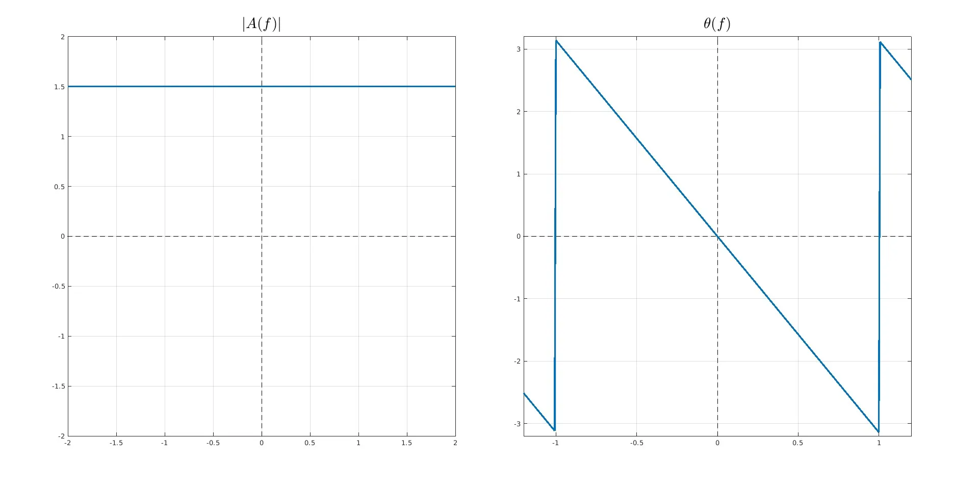
$$y(t)=k\cdot x(t-t_0),\quad \forall k, t_0\in \R;\,k\neq 0$$

Nel campo dei sistemi LTI, la condizione di non distorsione nel dominio delle frequenze è:

$$\begin{aligned} H(f)&=ke^{-j2\pi ft_0} \quad \forall f \in B_x=\{f:X(f)\neq 0\} \\ & \implies \begin{cases} A(f) = |k|\\ \Theta(f) = -2\pi f t_0 \end{cases} \end{aligned}$$

Dati $k=1.5$ e $t_0=0.5$ si ottengono i seguenti grafici. Si nota che, al di fuori del dominio $B_x$, le funzioni possono assumere un comportamento differente da quello indicato dalla formula soprastante. In questo caso $B_x = [-1\;1]$.

---

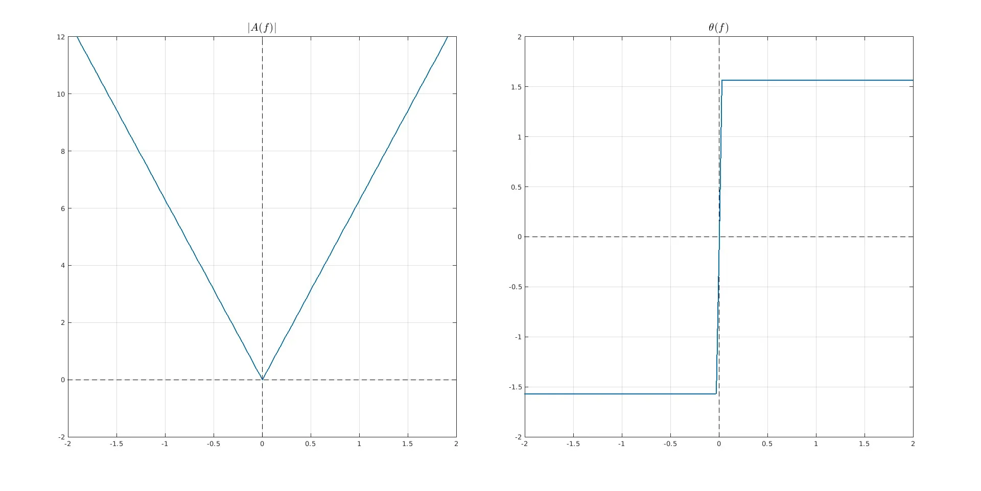
Esempio: data la trasformazione $\mathcal{T} = d/dt$, ovvero l’operatore di derivazione:

$$\begin{aligned} \Large \xrightarrow{x(t)} \boxed{\frac{d}{dt}} \xrightarrow{y(t)}\\ y(t)=\frac{d}{dt}x(t) \xrightarrow{\mathcal{F}}Y(f)=X(f)\cdot j2\pi f \end{aligned}$$

La risposta in frequenza è:

$$\begin{aligned} & H(f)=j2\pi f\\ & \implies \begin{cases} A(f)=2\pi |f|\\ \Theta(f)= \begin{cases}\pi/2 \quad &f>0\\ -\pi/2 \quad &f<0 \end{cases} \end{cases} \end{aligned}$$

I grafici si ottengono con il seguente codice MATLAB:

f_lim=15; f=linspace(-f_lim, f_lim, 1001); zero_values=zeros(length(f));
H_f=1j*2*pi.*f; % frequency response
A_f=abs(H_f);  % amplitude of H(f)
Theta_f=angle(H_f); % argument of H(f)

tiledlayout(1, 2); nexttile
plot(zero_values,f,'--',f, zero_values,'--',Color="black")
hold on; plot(f,A_f,LineWidth=1.5)
grid on; xlim([-2 2]); ylim([-2 12])
title({'$|A(f)|$'},'Interpreter','latex','FontSize',16)

nexttile
plot(zero_values,f,'--',f,zero_values,'--',Color="black")
hold on; plot(f,Theta_f, LineWidth=1.5)
grid on; xlim([-2 2]); ylim([-2 2])
title({'$\Theta(f)$'},'Interpreter','latex','FontSize',16)

Per la maggior parte dei segnali, il sistema che applica la derivazione è distorcente.

Sistemi non lineari

$$\Large \xrightarrow[\text{ (INPUT) }]{x(t)} \boxed{g[\cdot]} \xrightarrow[\text{ (OUTPUT) }]{y(t)}$$

I sistemi non lineari sono stazionari ed istantanei. L’output è nella forma:

$$y(t)=g[x(t)]$$

con $g(x)$ caratteristica di non linearità.

Il sistema è non lineare: non vale il principio di sovrapposizione degli effetti.

$$g(t)=\alpha x_1(t) + \beta x_2(t) \centernot\implies y(t)=\alpha g[x_1(t)] +\beta g[x_2(t)]$$

Il sistema è stazionario:

$$y(t) = g[x(t)] \implies g[x(t-t_0)] = y(t-t_0)$$

Il sistema è istantaneo o senza memoria:

$$y(t) = g[x(\alpha), \, \alpha = t]$$

Misura della distorsione

Dato l’input di riferimento $x(t)=a \cos(2\pi f_0 t)$ con periodo $T_0 = 1/f_0$.

L’output è $y(t)=g[a\cos(2\pi f_0 t)]$. I coefficienti della relativa serie di Fourier sono:

$$\large Y_k = \frac{1}{T_0} \int_{-T_0/2}^{T_0/2} g[x(t)]e^{-j2\pi k t/T_0}dt \quad \forall k$$

Ad ogni coppia di coefficienti $\pm k$ si associa la componente:

$$2|Y_k|\cos(2\pi k f_0 t + \arg(Y_k))$$

In $0$ si ha la componente continua, $2f_0,\;3f_0,\;\dots$ sono componenti di distorsione.

Il coefficiente di distorsione armonica di ordine $k$ è dato da:

$$D_k = \sqrt{\frac{P_k}{P_1}}= \sqrt{\frac{(2|Y_k|)^2/2}{(2|Y_1|)^2/2}}=\frac{|Y_k|}{|Y_1|}$$

Distorsione armonica totale

La total harmonic distortion è definita come:

$$\text{THD} = \sqrt{\frac{\sum_{k=2}^\infty P_k}{P_1}} = \sqrt{\sum_{k=2}^\infty\frac{|Y_k|^2}{|Y_1|^2}} = \sqrt{\sum_{k=1}^\infty D_k^2} = \sqrt{\frac{P_k-P_0-P_1}{P_1}} = \sqrt{\frac{P_k-Y_0^1}{2|Y_1|^2}-1}$$

Si noti che:

$$P_Y = P_0 + P_1 + \sum_{k=2}^\infty P_k \implies \sum_{k=2}^\infty P_k = P_Y-P_0-P_1$$

Esempio di sistema non lineare

Si consideri un sistema non lineare con ingresso $x(t)$, uscita $y(t)$ e caratteristica di non linearità data da:

$$y = g(x) = Au(x)$$

dove $u(\cdot)$ è la funzione gradino unitario e $A = 8$​ (numero puro).

Si richiede di effettuare il grafico del segnale in uscita quando l’input è:

$$x(t) = \cos(2\pi t / T_0)$$

e di determinare lo spettro di ampiezza di $y(t)$​.

Il gradino unitario annulla la funzione per $x(t)<0$.

Parte 1: Definire formalmente il segnale di uscita.

Bisogna determinare per quali valori di $t$ si ha $x(t)>0$.

Per la sola circonferenza goniometrica, ovvero per il dominio $[-1,1]$ si può scrivere:

$$\begin{aligned} & \cos(\alpha)>0\quad\forall -\pi/2 <\alpha <\pi/2 \\ & \implies x(t)>0\implies \cos(2\pi t/T_0)>0 \\ & \implies -\frac{\pi}{2}<\frac{2\pi}{T_0}t<\frac{\pi}{2}\\ & \implies -\frac{\pi}{2}\frac{T_0}{2\pi}<t<\frac{\pi}{2}\frac{T_0}{2\pi}\\ & \implies -\frac{T_0}{4}<t<\frac{T_0}{4} \end{aligned}$$

Dato $k\in\Z$, si può espandere il dominio di $t$ a tutto $\R$. Dunque, l’output del sistema è:

$$\begin{aligned} y(t) &= g\big(x(t)\big) = Au\big(x(t)\big) =\\ &= \begin{cases} A \quad & x(t) > 0\\ 0 \quad & x(t) < 0 \end{cases}\\ &= \begin{cases} A \quad & -T_0/4+2\pi k < t < T_0/4+2\pi k\\ 0 \quad & t < -T_0/4+2\pi k \land t > T_0/4+2\pi k \end{cases}\\ &= \begin{cases} A \quad & |t| < T_0/4+2\pi k\\ 0 \quad & |t| > T_0/4+2\pi k\\ \end{cases}\\ &= \sum_{k=-\infty}^{+\infty} A \;\text{rect} \bigg(\frac{t-k T_0}{T_0/2} \bigg) \end{aligned}$$

Dunque l’output è un segnale continuo e periodico costituito da rettangoli alti A e lunghi $T_0/2$​.

Dalla definizione soprastante si ha che:

$$-T_0/4 < t < T_0/4 \implies |t| < T_0/4$$

Per poter scrivere un dominio di t più comprensibile, si calcola il rettangolo nel caso in cui $k=0$ e si trasla. Si può procedere con le seguenti implicazioni:

$$\begin{aligned} & \text{rect}(t) = \begin{cases} 0 & \quad |t| > 1/2 \\ 1 & \quad |t| < 1/2 \\ 1/2 & \quad |t| = 1/2 \end{cases} \approx \begin{cases} 0 & \quad |t| \geq 1/2 \\ 1 & \quad |t| < 1/2 \end{cases}\\ & \text{rect}\bigg(\frac{t}{T_0/2} \bigg) = \begin{cases} 0 & \quad |t/(T_0/2)| \geq 1/2 \\ 1 & \quad |t/(T_0/2)| < 1/2 \end{cases} \\ \\ \implies & \bigg|\frac{t}{T_0/2}\bigg| < \frac{1}{2} \implies \frac{2}{T_0}|t| < \frac{1}{2} \implies \frac{T_0}{2}\frac{2}{T_0}|t| < \frac{1}{2}\frac{T_0}{2} \\ \implies & |t| < T_0/4 \end{aligned}$$

Per includere in $y(t)$ tutti gli altri rettangoli basta traslare a destra $\text{rect}\Big(t / (T_0/2)\Big)$ di $kT_0$ per ogni $k \in \Z$.

Grazie alla teoria delle ripetizioni periodiche, si può scrivere:

$$\begin{aligned} \widetilde{y}(t) &= A \;\text{rect} \bigg(\frac{t}{T_0/2} \bigg)\\ y(t) &= \sum_{n=-\infty}^{\infty} \widetilde{y}(t-nT_0) \\ & \implies Y_k = \frac{1}{T_0} \widetilde{Y}\bigg(\frac{k}{T_0}\bigg) \\ \end{aligned}$$

Poiché la trasformata di Fourier del rettangolo è il seno cardinale, i coefficienti della serie sono:

$$\begin{aligned} Y_k &= \frac{1}{T_0} \widetilde{Y}\bigg(\frac{k}{T_0}\bigg)=\\ &= \frac{1}{T_0} 2 T_0 \text{sinc}\bigg(\frac{T_0}{2} \frac{k}{T_0}\bigg)=\\ &= 2 \,\text{sinc}\bigg(\frac{k}{2} \bigg) \end{aligned}$$

Per determinare lo spettro di ampiezza di $y(t)$​ si studia il comportamento dei coefficienti per alcuni valori di k:

$$\begin{aligned} k=0 & \longrightarrow Y_0 =2\;\text{sinc}(0)=2\\ k=1 & \longrightarrow Y_1 =2\;\text{sinc}(1/2)=4 / \pi\\ k=2 & \longrightarrow Y_2 =2\;\text{sinc}(1) = 0 \\ k=3 & \longrightarrow Y_3 =-\frac{4}{3\pi}\\ k=4 & \longrightarrow Y_4 =0\\ \end{aligned}$$

Sia $Y_k^*$ il complesso coniugato di $Y_k$, poiché $y(t) \in \R$ (è una funzione a valori reali), allora vale $Y_{-k}=Y_k^*$ e quindi valgono anche le seguenti implicazioni:

1. il modulo (ampiezza) è simmetrico rispetto a $k$
   $|Y_{-k}|=|Y_k^*|$
2. gli argomenti (fasi) sono asimmetrici rispetto a $k$
   $\arg(Y_{-k})=-\arg(Y_{k})$

Sistemi LTI multivariabile

Questo argomento è analizzato nello specifico in un articolo dedicato: sistemi LTI multivariabile.